
Back when weights were outrageously interpretable
Hinton looks at palindromic vectors like (1,0,0,1,1,0,0,1)

“Learning representations by back-propagating errors” is the best introduction to neural networks I’ve read. I’m gutted it wasn’t in the ARENA curriculum or on the Ilya list. Their simple two-layer architecture learns some extraordinarily interpretable weights.
If you’re just interested in seeing these interpretable weights, you can just read ‘Dataset’ and ‘The interpretable learned weights’.
Let’s get right into it!
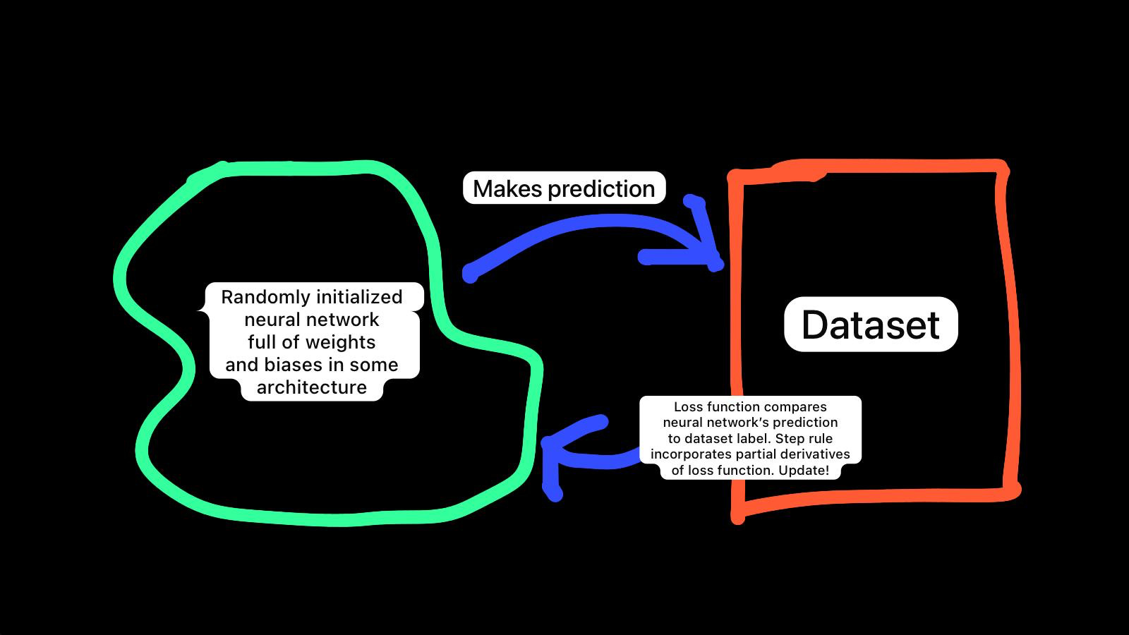
Training = Architecture at initialization + Dataset + Loss function + Step rule
Architecture at initialization
This is a one-hidden-layer neural network with two units in the hidden layer. It takes a six-bit vector as input and outputs a scalar.

Weights (biases are weights like any other!) are initialized with values randomly drawn from uniform distribution U(-0.3, 0.3).

                   ( output layer )

                     [ y_out ] ∈ (0,1)
                     (σ node)
                     bias b_out ∈ U(-0.3, 0.3)
                           ^
                         /   \
                        /     \
     w_out_L ∈ U(-0.3,0.3)   w_out_R ∈ U(-0.3,0.3)
                      /         \
                     /           \
                 [ h_L ]        [ h_R ]
                   (σ)            (σ)
   bias b_L ∈ U(-0.3,0.3)   bias b_R ∈ U(-0.3,0.3)
   ^   ^   ^   ^   ^   ^       ^   ^   ^   ^   ^   ^
   |   |   |   |   |   |       |   |   |   |   |   |
   |   |   |   |   |   |       |   |   |   |   |   |
   w_L1 ∈ U(-0.3,0.3)          w_R1 ∈ U(-0.3,0.3)
   w_L2 ∈ U(-0.3,0.3)          w_R2 ∈ U(-0.3,0.3)
   w_L3 ∈ U(-0.3,0.3)          w_R3 ∈ U(-0.3,0.3)
   w_L4 ∈ U(-0.3,0.3)          w_R4 ∈ U(-0.3,0.3)
   w_L5 ∈ U(-0.3,0.3)          w_R5 ∈ U(-0.3,0.3)
   w_L6 ∈ U(-0.3,0.3)          w_R6 ∈ U(-0.3,0.3)

          ( input layer, type annotations )

    x1        x2        x3        x4        x5        x6
  [bit]     [bit]     [bit]     [bit]     [bit]     [bit]
  ∈{0,1}    ∈{0,1}    ∈{0,1}    ∈{0,1}    ∈{0,1}    ∈{0,1}

The same 6-bit input vector is fed in twice, once into each hidden unit. That's just how feedforward networks / fully-connected layers work: each hidden unit sees the whole input vector.
Dataset
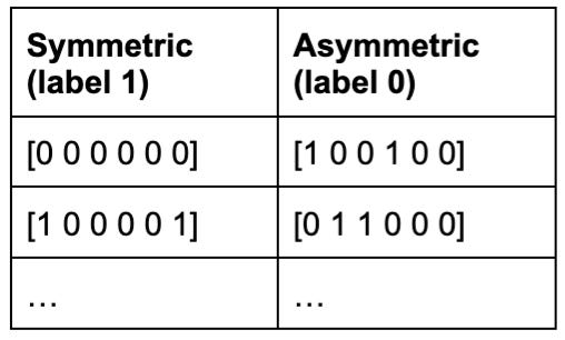
64 six-bit vectors. Of these, eight are symmetric1 and given ground-truth output label ‘1’. The other 56 are given ground-truth output label ‘0’.
Loss Function
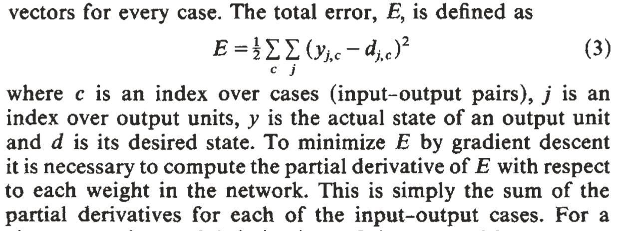
Step rule
Per-weight update = (Learning rate * Gradient) + Momentum

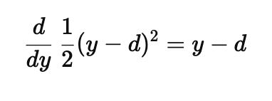
Since there’s only one hidden layer, calculating the gradient (partial derivative of error wrt weight) is super easy—just two applications of the chain rule:
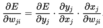
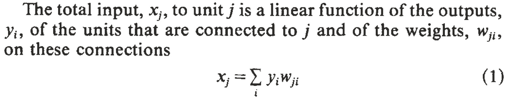
xj, yj, and wji were defined as follows:
Thanks to the following three facts, we get a very clean expression:
the cute, calculus-simplifying 1/2 scaling discussed earlier
the fact that yj is output of a sigmoid activation function, and the sigmoid’s derivative can be written in terms of its output: yj (1-yj)
yi being coefficient on weight wji in linear combination (1)
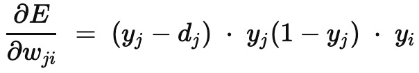
You can now sub this into the step rule and we’re away.
Train, train, train!
They trained the network for 1425 sweeps over the 64-element dataset: each data point was seen ~22 times. (Perhaps a higher learning rate could’ve enabled slightly less sweeps).
How many times do current frontier LLMs see each data point? For EleutherAI’s Pythia, trained on the Pile, the answer seems to be 1-2x:
“each model saw 299,892,736,000 ≈ 300B tokens… just under 1 epoch on the Pile for ‘standard’ models, and ≈ 1.5 epochs on the deduped Pile.”
The answer probably varies with data point quality.
The interpretable learned weights
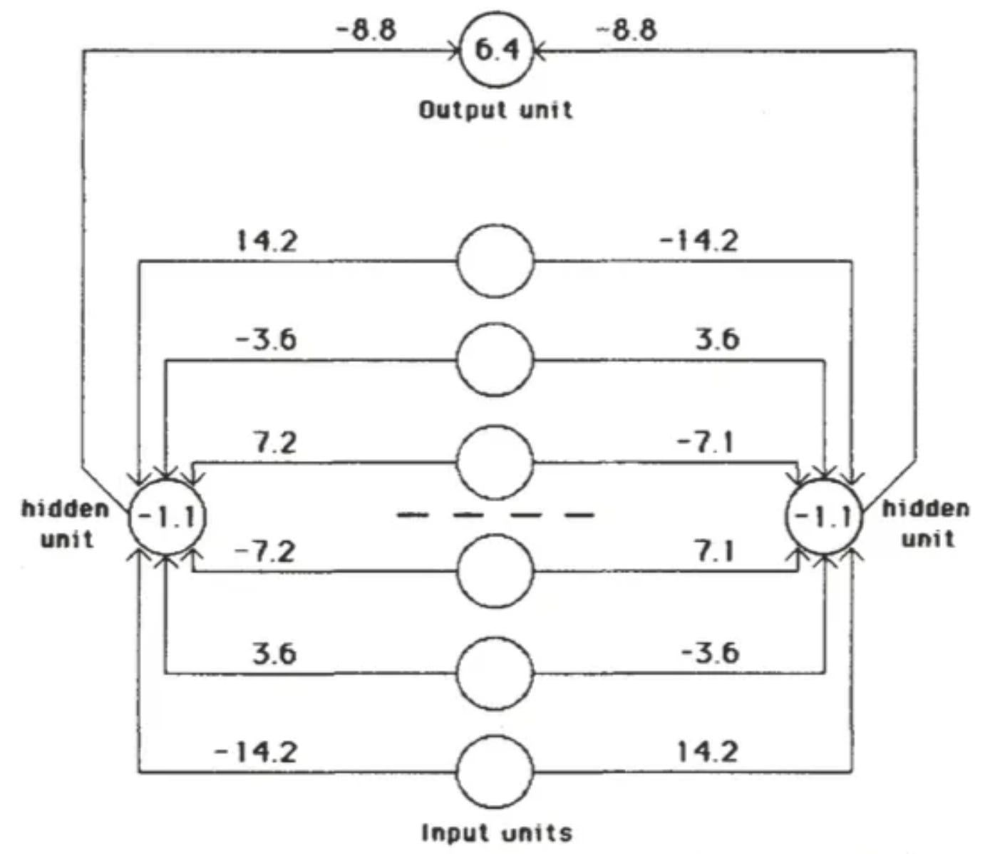
Symmetry
Whoa! These weights are…symmetric?
That’s right: the weights into Left Hidden Unit literally take form:
w0, w1, w2, -w2, -w1, -w0
with mirrored weights heading into Right Hidden Unit.
The key property of this solution is that for a given hidden unit, weights that are symmetric about the middle of the input vector are equal in magnitude and opposite in sign. So if a symmetrical pattern is presented, both hidden units will receive a net input of 0 from the input units, and, because the hidden units have a negative bias, both will be off. In this case the output unit, having a positive bias, will be on.
Ratio 1:2:4
Not only are they symmetric, but they’re in ratio 1 : 2 : 4!
Note that the weights on each side of the midpoint are in the ratio 1:2:4. This ensures that each of the eight patterns that can occur above the midpoint sends a unique activation sum to each hidden unit, so that the only pattern below the midpoint that can exactly balance this sum is the symmetrical one.
Why 1:2:4? Well, this is 2^0 : 2^1 : 2^2. You can work in base-k to ensure there’s no interference between indices of distinct k, and k = 2 is simplest.
How on earth did the neural network learn this simplest solution? :D
Gradient Descent Biased Towards Simplest Solution
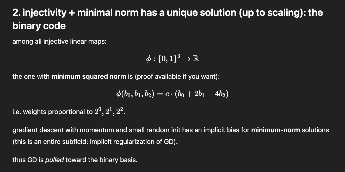
The particular learned weights (14.2, -3.6, 7.2) seem to be an artifact of the random initialization. You’d get different weights w0, w1, w2 if you re-ran this, but they’d still be in some permutation of 1:2:4 because this is the minimum-norm solution for an injective map from bits to scalar.
Coming Soon
We’ve now seen that “Learning representations by back-propagating errors” might as well be called “Learning interpretable representations by back-propagating errors over simple synthetic datasets.”
I might talk about the second task covered in the paper, which features family trees.
But really, this entire paper exegesis was motivated by an investigation for another blog post I’m writing: What actually happens in an ML training step, and is this process best represented by a bidirectional or unidirectional arrow? I expect I’ll publish that later this week.
Think about it: these are uniquely determined by the first three bits, for which there are 2^3 = 8 possibilities.